Display Code
knitr::opts_chunk$set(warning = FALSE, message = FALSE)

library(tidyverse)
library(janitor)
library(here)
library(readxl)The United States Geological Survey (USGS) has reported daily water use since as early as the 1950s. There is a plethora of knowledge that you are able to extract in each of these databases, indubitably. For this case study, I will examine daily freshwater withdrawal trends across sector, state, and source.
In this analysis, I used the tidyverse, janitor, here, and readxl packages.
knitr::opts_chunk$set(warning = FALSE, message = FALSE)
library(tidyverse)
library(janitor)
library(here)
library(readxl)These data sets contain all freshwater and saline withdrawals across sector in the United States. In order to effectively join each dataset as a dataframe, we must validate the columns using the correct metadata for each file containing 5 year data. See Table 1 for matching keys.
Table 1: “Sets” of data, for which each of the sets have ALL column tags in common. Data from USGS (1950-2015). The data for this project are available from the United States Geological Survey for years 1950-2015.
| year | public supply | irrigation | rural | industrial | thermo | state |
|---|---|---|---|---|---|---|
| 1950-1955 | ps_wgw_fr + ps_wsw_fr | ir_wgw_fr + ir_wsw_fr | NA | inpt_wgw_fr + inpt_wsw_fr | NA | area |
| 1960-1980 | ps_wgw_fr + ps_wgw_fr | ir_wgw_fr + ir_wsw_fr | do_wgw_fr + do_wsw_fr + ls_wgw_fr + ls_wsw_fr | oi_wgw_fr + oi_wsw_fr | pt_wgw_fr + pt_wsw_fr | area |
| 1985-1990 | ps_wgwfr + ps_wswfr | ir_wgwfr + ir_wswfr | do_ssgwf + do_ssswf + ls_gwtot + ls_swtot | in_wgwfr + in_wswfr + mi_wgwfr + mi_wswfr | pt_wgwfr + pt_wswfr | scode |
| 1995 | ps_wgw_fr + ps_wsw_fr | ir_wgw_fr + ir_wsw_fr | do_wgw_fr + do_wsw_fr + ls_wgw_fr + ls_wsw_fr | in_wgw_fr + in_wsw_fr + mi_wgw_fr + mi_wsw_fr | pt_wgw_fr + pt_wsw_fr | state_code |
| 2000 | ps_wgw_fr + ps_wsw_fr | it_wgw_fr + it_wsw_fr | do_wgw_fr + do_wsw_fr + ls_wgw_fr + ls_wsw_fr | in_wgw_fr + in_wsw_fr + mi_wgw_fr + mi_wsw_fr | pt_wgw_fr + pt_wsw_fr | statefips |
| 2005 | ps_wgw_fr + ps_wsw_fr | ir_wgw_fr + ir_wsw_fr | do_wgw_fr + do_wsw_fr + ls_wgw_fr + ls_wsw_fr | in_wgw_fr + in_wsw_fr + mi_wgw_fr + mi_wsw_fr | pt_wgw_fr + pt_wsw_fr | state_fips |
| 2010 - 2015 | ps_wgw_fr + ps_wsw_fr | ir_wgw_fr + ir_wsw_fr | do_wgw_fr + do_wsw_fr + li_wgw_fr + li_wsw_fr | in_wgw_fr + in_wsw_fr + mi_wgw_fr + mi_wsw_fr | pt_wgw_fr + pt_wsw_fr | statefips |
For this step, you will see that I use lapply() repeatedly for each file that I want to read in as a dataframe. I am able to call the file path using `here()’, looping through each sheet and skipping the first 3 rows for most of the datasheets. See code below to see where there are discrepancies to the file convention. This is how we begin to fix messy data! ☺
Following this, I reduce each sheet to one data frame, joining by Area. Now we are in business. Now that each of our dataframes are formatted the same, I can mutate each of the withdrawal columns to be numeric for calculations and viz later down the road.
#List all files in data folder
list.files(path = ("/Users/bgrazda/Desktop/Rprojects/water_use_1950_2015/data"))character(0)#Read data file for 1950
d_1950 <- lapply(excel_sheets(here("data/us1950.xlsx")), function(x) read_excel(here("data/us1950.xlsx"), skip = 3, sheet = x)) |> #loops through the name of sheets, reads in the data within a given sheet, skips line 3, loops through sheet x
reduce(left_join, by = "Area") |> #Each sheet has area, joins sheets into one df
clean_names() |> #snake case
select(!"note_industrial_and_thermoelectric_were_combined_in_1950") |> #removes not needed column
mutate_at(vars(2:8), as.numeric, na.rm = TRUE ) #turns into numerics, excludes area code as char
#Read data file for 1955
d_1955 <- lapply(excel_sheets(here("data/us1955.xlsx")), function(x)read_xlsx(here("data/us1955.xlsx"), skip = 3, sheet = x)) |>
reduce(left_join, by = "Area") |>
clean_names() |>
select(!"note_industrial_and_thermoelectric_were_combined_in_1955") |> #remove not needed columns
mutate_at(vars(2:10), as.numeric, na.rm = TRUE) #mutate to numerics
#Read data file for 1960
d_1960 <- lapply(excel_sheets(here("data/us1960.xlsx")), function(x)read_xlsx(here("data/us1960.xlsx"), skip = 3, sheet = x)) |>
reduce(left_join, by = "Area") |>
clean_names() |>
mutate_at(c(2:35), as.numeric, na.rm = TRUE) #mutates to numerics
#Read data file for 1965
d_1965 <- lapply(excel_sheets(here("data/us1965.xlsx")), function(x)read_xlsx(here("data/us1965.xlsx"), skip = 3, sheet = x)) |>
reduce(left_join, by = "Area") |>
clean_names() |>
mutate_at(c(2:33), as.numeric, na.rm = TRUE) #mutate to numerics
#Read data file for 1970
d_1970 <- lapply(excel_sheets(here("data/us1970.xlsx")), function(x)read_xlsx(here("data/us1970.xlsx"), skip = 3, sheet = x)) |>
reduce(left_join, by = "Area") |>
clean_names() |>
slice(1:53) |> #slice to omit last row
mutate_at(c(2:34), as.numeric, na.rm = TRUE) #mutate to numerics, keep char for area
#Read data file for 1975
d_1975 <- lapply(excel_sheets(here("data/us1975.xlsx")), function(x)read_xlsx(here("data/us1975.xlsx"), skip = 3, sheet = x)) |>
reduce(left_join, by = "Area") |>
clean_names() |>
mutate_at(c(2:34), as.numeric, na.rm = TRUE) #change to numerics, keep area as a character
#Read data file for 1980
d_1980 <- lapply(excel_sheets(here("data/us1980.xlsx")), function(x)read_xlsx(here("data/us1980.xlsx"), skip = 3, sheet = x)) |>
reduce(left_join, by = "Area") |>
clean_names() |>
mutate_at(c(2:34), as.numeric, na.rm = TRUE) #change to numerics, keep area as a character
#Read data file for 1985
d_1985 <- read_delim(here("data/us1985.txt"), delim = "\t") |>
clean_names() |> #no need to lapply, all txt file already there
mutate_at(c(2, 6:163), as.numeric, na.rm = TRUE) #mutate to numeric, include year
#Read data file for 1990
d_1990 <- read_xls(here("data/us1990.xls")) |>
clean_names() |>
slice_head(n = 3225) |> #omits the last row that contains NA, initially 3226 variables
mutate_at(c(2, 6:163), as.numeric, na.rm = TRUE) #change to numerics, keep scode as a character, year as numeric
#Read data file for 1995
d_1995 <- read_xls(here("data/us1995.xls")) |>
clean_names() |>
mutate_at(c(1, 6:252), as.numeric, na.rm = TRUE) #change to numerics, state_code is character, year
#Read data file for 2000
d_2000 <- read_xls(here("data/us2000.xls")) |>
clean_names() |>
mutate_at(c(5:70), as.numeric, na.rm = TRUE) #change to numerics
#Read data file for 2005
d_2005 <- read_xls(here("data/us2005.xls")) |>
clean_names() |>
mutate_at(c(6:108), as.numeric, na.rm = TRUE) #change to numerics
#Read data file for 2010
d_2010 <- read_xlsx(here("data/us2010.xlsx")) |>
clean_names() |>
mutate_at(c(6:117), as.numeric, na.rm = TRUE) #change to numerics
#Read data file for 2015
d_2015 <- read_xlsx(here("data/us2015.xlsx"), skip = 1) |>
clean_names() |>
mutate_at(c(6:141), as.numeric, na.rm = TRUE) #change to numericsGreat! Each of our dataframes have the correct data type for the columns of interest, however, our column names are all over the place. As seen in Table 1, the naming conventions for our sector measurements has not been reproducible for every year since 1950. Using the predetermined keys from the metadata, we can mutate the columns for each sector that withdraws freshwater, removing NAs as we go. I selected every 5th year to visualize incremental trends. Last step here is to pivot longer. Now our data is happily tidy!
#assign new variables
wu_1950 <- d_1950 |> #calls the year 1950
select("area", contains(c("wsw_fr", "wgw_fr"))) |> #copies necessary columns, excludes saline withdrawal
mutate(public_supply = ps_wsw_fr + ps_wgw_fr, #sum public supply columns
irrigation = ir_wgw_fr + ir_wsw_fr, #sum irrigation columnes
rural = NA, #sum rural columns except its NA
industrial = inpt_wgw_fr + inpt_wsw_fr, #sum industrial columns
thermoelectric = NA, #thermoelectric columns except NA
state = area, na.rm = TRUE) |> #reassign area to state
select("public_supply", "irrigation", "rural", "industrial", "thermoelectric", "state") |> #select only the columns i want
mutate(year = 1950) |>
pivot_longer(cols = 1:5, names_to = "sector", values_to = "withdrawals")
wu_1955 <- d_1955 |> #year!
select("area", contains(c("wsw_fr", "wgw_fr"))) |> #copies necessary columns, excludes saline withdrawal
mutate(public_supply = ps_wsw_fr + ps_wgw_fr, #sum public supply columns
irrigation = ir_wgw_fr + ir_wsw_fr, #sum irrigation columnes
rural = NA, #sum rural columns except its NA
industrial = inpt_wgw_fr + inpt_wsw_fr, #sum industrial columns
thermoelectric = NA, #thermoelectric columns except NA
state = area, na.rm = TRUE) |> #reassign area to state
select("public_supply", "irrigation", "rural", "industrial", "thermoelectric", "state") |> #select only the columns i want
mutate(year = 1955) |>
pivot_longer(cols = 1:5, names_to = "sector", values_to = "withdrawals")
wu_1960 <- d_1960 |> #year!
mutate(public_supply = ps_wsw_fr + ps_wgw_fr, #sum public supply columns
#totsl irrigation withdrawals since lack of data that was making my ggplot look funny before
irrigation = ir_w_fr_to, #sum irrigation columnes
rural = do_wgw_fr + do_wsw_fr + ls_wgw_fr + ls_wsw_fr, #sum rural columns except its NA
industrial = oi_wgw_fr + oi_wsw_fr, #sum industrial columns
thermoelectric = pt_wgw_fr + pt_wsw_fr, #thermoelectric columns except NA
state = area, na.rm = TRUE) |> #reassign area to state
select("public_supply", "irrigation", "rural", "industrial", "thermoelectric", "state") |> #select only the columns i want
mutate(year = 1960) |>
pivot_longer(cols = 1:5, names_to = "sector", values_to = "withdrawals")
wu_1965 <- d_1965 |> #year!
select("area", contains(c("wsw_fr", "wgw_fr"))) |> #copies necessary columns, excludes saline withdrawal
mutate(public_supply = ps_wsw_fr + ps_wgw_fr, #sum public supply columns
irrigation = ir_wgw_fr + ir_wsw_fr, #sum irrigation columnes
rural = do_wgw_fr + do_wsw_fr + ls_wgw_fr + ls_wsw_fr, #sum rural columns except its NA
industrial = oi_wgw_fr + oi_wsw_fr, #sum industrial columns
thermoelectric = pt_wgw_fr + pt_wsw_fr, #thermoelectric columns
state = area, na.rm = TRUE) |> #reassign area to state
select("public_supply", "irrigation", "rural", "industrial", "thermoelectric", "state") |> #select only the columns i want
mutate(year = 1965) |>
pivot_longer(cols = 1:5, names_to = "sector", values_to = "withdrawals")
wu_1970 <- d_1970 |> #year!
select("area", contains(c("wsw_fr", "wgw_fr"))) |> #copies necessary columns, excludes saline withdrawal
mutate(public_supply = ps_wsw_fr + ps_wgw_fr, #sum public supply columns
irrigation = ir_wgw_fr + ir_wsw_fr, #sum irrigation columnes
rural = do_wgw_fr + do_wsw_fr + ls_wgw_fr + ls_wsw_fr, #sum rural columns
industrial = oi_wgw_fr + oi_wsw_fr, #sum industrial columns
thermoelectric = pt_wgw_fr + pt_wsw_fr, #thermoelectric columns
state = area, na.rm = TRUE) |> #reassign area to state
select("public_supply", "irrigation", "rural", "industrial", "thermoelectric", "state") |> #select only the columns i want
mutate(year = 1970) |>
pivot_longer(cols = 1:5, names_to = "sector", values_to = "withdrawals")
wu_1975 <- d_1975 |> #year!
select("area", contains(c("wsw_fr", "wgw_fr"))) |> #copies necessary columns, excludes saline withdrawal
mutate(public_supply = ps_wsw_fr + ps_wgw_fr, #sum public supply columns
irrigation = ir_wgw_fr + ir_wsw_fr, #sum irrigation columnes
rural = do_wgw_fr + do_wsw_fr + ls_wgw_fr + ls_wsw_fr, #sum rural columns
industrial = oi_wgw_fr + oi_wsw_fr, #sum industrial columns
thermoelectric = pt_wgw_fr + pt_wsw_fr, #thermoelectric columns
state = area, na.rm = TRUE) |> #reassign area to state
select("public_supply", "irrigation", "rural", "industrial", "thermoelectric", "state") |> #select only the columns i want
mutate(year = 1975) |>
pivot_longer(cols = 1:5, names_to = "sector", values_to = "withdrawals")
wu_1980 <- d_1980 |> #year!
select("area", contains(c("wsw_fr", "wgw_fr"))) |> #copies necessary columns, excludes saline withdrawal
mutate(public_supply = ps_wsw_fr + ps_wgw_fr, #sum public supply columns
irrigation = ir_wgw_fr + ir_wsw_fr, #sum irrigation columns
rural = do_wgw_fr + do_wsw_fr + ls_wgw_fr + ls_wsw_fr, #sum rural columns
industrial = oi_wgw_fr + oi_wsw_fr, #sum industrial columns
thermoelectric = pt_wgw_fr + pt_wsw_fr, #thermoelectric columns
state = area, na.rm = TRUE) |> #reassign area to state
select("public_supply", "irrigation", "rural", "industrial", "thermoelectric", "state") |> #select only the columns i want
mutate(year = 1980) |>
pivot_longer(cols = 1:5, names_to = "sector", values_to = "withdrawals")
wu_1985 <- d_1985 |>
select("scode", contains(c("sw", "gw"))) |>
mutate(public_supply = ps_wswfr + ps_wgwfr, #sum public supply columns
irrigation = ir_wgwfr + ir_wswfr, #sum irrigation columnes
rural = do_ssgwf + do_ssswf + ls_gwtot + ls_swtot, #sum rural columns
industrial = in_wgwfr + in_wswfr + mi_wgwfr + mi_wswfr, #sum industrial columns
thermoelectric = pt_wgwfr + pt_wswfr, #thermoelectric columns
state = scode, na.rm = TRUE) |> #reassign area to state
select("public_supply", "irrigation", "rural", "industrial", "thermoelectric", "state") |> #select only the columns i want)
group_by(state) |> #looks at state column and groups values
summarize_at(c(1:5), sum) |> #sum up the states
ungroup() |> #ungroups to prevent errors
mutate(year = 1985) |>
pivot_longer(cols = 2:6, names_to = "sector", values_to = "withdrawals")
wu_1990 <- d_1990 |>
select("scode", contains(c("sw", "gw"))) |>
mutate(public_supply = ps_wswfr + ps_wgwfr, #sum public supply columns
irrigation = ir_wgwfr + ir_wswfr, #sum irrigation columnes
rural = do_ssgwf + do_ssswf + ls_gwtot + ls_swtot, #sum rural columns
industrial = in_wgwfr + in_wswfr + mi_wgwfr + mi_wswfr, #sum industrial columns
thermoelectric = pt_wgwfr + pt_wswfr, #thermoelectric columns
state = scode, na.rm = TRUE) |> #reassign area to state
select("public_supply", "irrigation", "rural", "industrial", "thermoelectric", "state") |> #only wanted values
group_by(state) |> #looks at state column and groups values
summarize_at(c(1:5), sum) |> #sum up the states
ungroup() |> #ungroups to prevent errors
mutate(year = 1990) |>
pivot_longer(cols = 2:6, names_to = "sector", values_to = "withdrawals")
wu_1995 <- d_1995 |>
select("state_code", contains(c("wgw_fr", "wsw_fr"))) |>
mutate(public_supply = ps_wsw_fr + ps_wgw_fr, #sum public supply columns
irrigation = ir_wgw_fr + ir_wsw_fr, #sum irrigation columnes
rural = do_wgw_fr + do_wsw_fr + ls_wgw_fr + ls_wsw_fr, #sum rural columns
industrial = in_wgw_fr + in_wsw_fr + mi_wgw_fr + mi_wsw_fr, #sum industrial columns
thermoelectric = pt_wgw_fr + pt_wsw_fr, #thermoelectric columns
state = state_code, na.rm = TRUE) |>
select("public_supply", "irrigation", "rural", "industrial", "thermoelectric", "state") |> #only wanted values
group_by(state) |> #looks at state column and groups values
summarize_at(c(1:5), sum) |> #sum up the states
ungroup() |> #no errors here no sir
mutate(year = 1995) |>
pivot_longer(cols = 2:6, names_to = "sector", values_to = "withdrawals")
wu_2000 <- d_2000 |>
select(statefips, contains(c("wgw_fr", "wsw_fr"))) |> #select these ones to narrow down
mutate(public_supply = ps_wgw_fr + ps_wsw_fr, #public supply sum column
irrigation = it_wgw_fr + it_wsw_fr, #irrigation summing columns
rural = do_wgw_fr + do_wsw_fr + ls_wgw_fr + ls_wsw_fr, #rural summing col
industrial = in_wgw_fr + in_wsw_fr + mi_wgw_fr + mi_wsw_fr, #industrial sum col
thermoelectric = pt_wgw_fr + pt_wsw_fr, #thermoelectric sum col
state = statefips, na.rm = TRUE) |> #state code is fips
select("public_supply", "irrigation", "rural", "industrial", "thermoelectric", "state") |>
group_by(state) |> #group states
summarize_at(c(1:5), sum) |> #selected columns
ungroup() |> #ungroup
mutate(year = 2000) |> #add column for 2000
pivot_longer(cols = 2:6, names_to = "sector", values_to = "withdrawals") #now only 4 columns
wu_2005 <- d_2005 |> #year of interest
select(statefips, contains(c("wgw_fr", "wsw_fr"))) |> #help search for wanted variables
mutate(public_supply = ps_wgw_fr + ps_wsw_fr, #sum up
irrigation = ir_wgw_fr + ir_wsw_fr, #irrigationsum
rural = do_wgw_fr + do_wsw_fr + ls_wgw_fr + ls_wsw_fr, #rural sum
industrial = in_wgw_fr + in_wsw_fr + mi_wgw_fr + mi_wsw_fr, #industrial sum
thermoelectric = pt_wgw_fr + pt_wsw_fr, #thermo sum
state = statefips, na.rm = TRUE) |> #state fips char and then ALL values na.rm = true
select("public_supply", "irrigation", "rural", "industrial", "thermoelectric", "state") |> #only want these
group_by(state) |>
summarize_at(c(1:5), sum) |>
ungroup() |>
mutate(year = 2005) |>
pivot_longer(cols = 2:6, names_to = "sector", values_to = "withdrawals") #same deal group sum then ungroup and add column to get 4 total
wu_2010 <- d_2010 |>
select(statefips, contains(c("wgw_fr", "wsw_fr"))) |>
mutate(public_supply = ps_wgw_fr + ps_wsw_fr,
irrigation = ir_wgw_fr + ir_wsw_fr,
rural = do_wgw_fr + do_wsw_fr + li_wgw_fr + li_wsw_fr,
industrial = in_wgw_fr + in_wsw_fr + mi_wgw_fr + mi_wsw_fr,
thermoelectric = pt_wgw_fr + pt_wsw_fr,
state = statefips, na.rm = TRUE) |>
select("public_supply", "irrigation", "rural", "industrial", "thermoelectric", "state") |> #after summing up correct columns, select them to get only these
group_by(state) |>
summarize_at(c(1:5), sum) |>
ungroup() |>
mutate(year = 2010) |>
pivot_longer(cols = 2:6, names_to = "sector", values_to = "withdrawals") #same deal group sum then ungroup and add column to get 4 total
wu_2015 <- d_2015 |>
select(statefips, contains(c("wgw_fr", "wsw_fr"))) |>
mutate(public_supply = ps_wgw_fr + ps_wsw_fr,
irrigation = ir_wgw_fr + ir_wsw_fr,
rural = do_wgw_fr + do_wsw_fr + li_wgw_fr + li_wsw_fr,
industrial = in_wgw_fr + in_wsw_fr + mi_wgw_fr + mi_wsw_fr,
thermoelectric = pt_wgw_fr + pt_wsw_fr,
state = statefips, na.rm = TRUE) |>
select("public_supply", "irrigation", "rural", "industrial", "thermoelectric", "state") |> #after summing up correct columns, select them to get only these
group_by(state) |>
summarize_at(c(1:5), sum) |>
ungroup() |>
mutate(year = 2015) |> #same deal group sum then ungroup and add column to get 4 total
pivot_longer(cols = 2:6, names_to = "sector", values_to = "withdrawals")Storing our water use data every 5 years gives us a lot of information, but not in the most convenient places. Luckily we just cleaned each of these data frames under the same conventions so we will be able to bind each dataframe into one mega water use dataframe using rbind(). This analysis excludes District of Columbia, Puerto Rico, and the Virgin Islands.
I was able to calculate the yearly number of withdrawals in the United States grouping different combinations of sector, sector & year, and year. This will help with visualizing different insights. I arranged the water use by sector data frame to help with plotting.
wu_all <- rbind(wu_1950, wu_1955, wu_1960, wu_1965, wu_1970, wu_1975, wu_1980, wu_1985,
                wu_1990, wu_1995, wu_2000, wu_2005, wu_2010, wu_2015, deparse.level = 1) |>    #all data binded
          filter(!state %in% c("11", "72", "78"))                               #filter out non states: DC, Puerto Rico, VI

wu_all_total <- wu_all |>                                  #call the previous data frame to make totals
               group_by(year) |>                            #combine by year
               summarize_at(vars("withdrawals"), sum, na.rm = TRUE) |>                            #we want to sum up all the withdrawals per year
               ungroup()                                                      #error prevention

wu_all_sector <- wu_all |>
                group_by(sector, year) |>                  #we want to add up all sectors by year
                summarize_at(vars("withdrawals"), sum, na.rm = TRUE) |>          #sum up withdrawals after grouping
                ungroup()                                #ungroup

wu_all_check <- wu_all_sector |>                         #3 columns
              group_by(sector) |>                        #we don't need to look at year
              summarize_at(vars("withdrawals"), sum, na.rm = TRUE) |>          #sum up withdrawals
              ungroup() |>                              #no errors
arrange(withdrawals) #arranges sectors in ascending order by total withdrawal; ggplot in next step is ordering the sector based on the total sectors for every year Using our good friend ggplot(), I plotted the water use data as a bar chart. This visualization seemed to make the most intuitive sense as far as showing water use by sector from 1950-2015.
ggplot() +
        geom_col(data = wu_all_sector, aes(x = year, y = withdrawals,               #data frame, x axis is year, y axis is withdrawal
                 fill = reorder(sector, withdrawals, decreasing = FALSE)),          #we want the sector to be reordered based on increasing withdrawals
                 position = position_dodge(3.5),                                   #dodgin bars for visualization
                 width = 4) +                                                     #thickness of bars
        scale_fill_manual(limits = c("rural", "public_supply", "industrial", "thermoelectric", "irrigation"), labels = c("Rural", "Public Supply", "Industrial", "Thermoelectric", "Irrigation"), values = c("#5ab4ac","#1f78b4", "#de2d26","#fc8d59", "#31a354" ))  +        #reassigns colors, gets rid of snake case legend
          geom_line(data = wu_all_total, aes(x = year, y= withdrawals/2),
                    size = 1,
                    colour = "grey") +               #line data in grey
          geom_point(data = wu_all_total, aes(x = year, y = withdrawals/2),
                    size = 2,
                    colour = "grey") +            #plots grey points on the line
                 #removes padding between first and last years (removes 1945 and 2020)
         scale_x_continuous(breaks = scales::pretty_breaks(n = 14), expand = c(0,0)) +     #breaks on the x axis
                 #removes padding between the x axis and the first plotted value
         scale_y_continuous(breaks = scales::pretty_breaks(n = 10), labels = scales::comma, limits = c(0, 200000), sec.axis = sec_axis(trans = ~.*2, breaks = scales::pretty_breaks(n = 10), name = "Total Withdrawals Mgal/Day", labels = scales::comma), expand = c(0,0)) +                       #sets right side secondary axis and names it with limits up to 200,000
          labs(x = " ", y = "Sector Withdrawals Mgal/day", title = "Freshwater withdrawals in the United States from 1950-2015", caption =  "Source: United States Geological Survey.", fill = "") +         #left axes title with labeling x axis and giving caption
      #classic theme removes gridlines and gives a white background
         theme_classic() +
         theme(legend.title = element_text(size = 10, color = "black"),                 #change legend size and color
                     legend.position = "bottom",                                       #change legend position to top
                      axis.text = element_text(size = 10, color = "black"),         #change axis text on the left and change color to black
                      axis.text.y.right = element_text(color = "grey"),           #put right axis text to be grey
                      axis.title.y.right = element_text(vjust = 2, color = "grey"),          #make right axis title grey
                      axis.title = element_text(size = 15),                     #change title size
                      plot.caption = element_text(hjust = -0.15, size = 16, face = "bold"))           #change caption positioning and size and face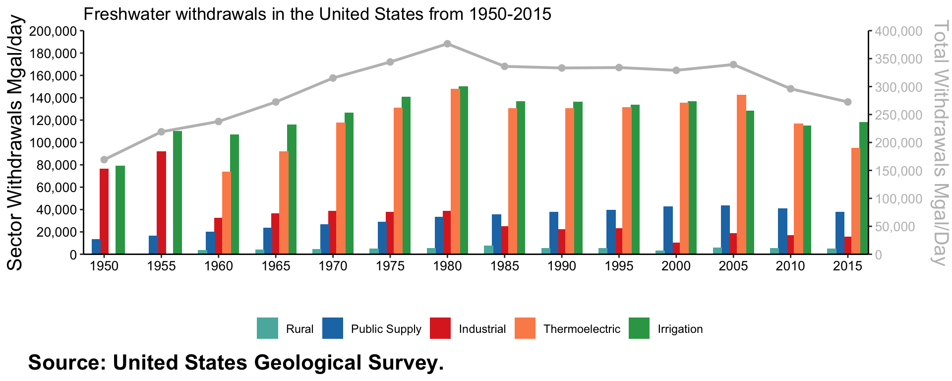
Note: In this USGS plot, thermoelectricity is shown to have the highest overall amount of freshwater withdrawals. This may be due in part to there being no indication of the type of water that is used. For example, this plot could account for both withdrawals and deliveries within the thermoelectric sector.
Total water withdrawals were increasing up until 1980, and then over time it has decreased. The two major sectors over time have been thermoelectric and irrigation for water withdrawals. 1980 had the greatest year of overall water consumption. Since then, we have improved water efficiency across all sectors. I was shocked to see how little the public supply sector uses water in comparison to other sectors!